Dispersion Correction
Several dispersion correction methods have been developed. Most of them describe dispersion as a convolution of the true concentration curve with a dispersion function, and correction amounts to a numerical deconvolution which produces results suffering from excessive noise. Munk et al. [1] have developed an alternative approach which circumvents numerical deconvolution. It describes transport of blood through a catheter by a "transmission-dispersion" model which includes two components: molecules which travel undisturbed in the inner of the catheter (convective flow), and molecules close to the catheter wall to which sticking occurs (stagnant flow).
The true (corrected) blood activity concentration CB(t) can be calculated from the measured concentration CmB(t) as follows.
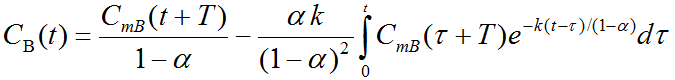
There are three parameters in the equation which are characteristic for the experimental acquisition setup:
▪the transit time T,
▪a parameter k[1/min] which refers to the stickiness of the catheter for a tracer, and
▪the stagnant fraction α. If α=0, no dispersion occurs, just a delay. α=1 is not allowed in the equation, so 0≤α<1.
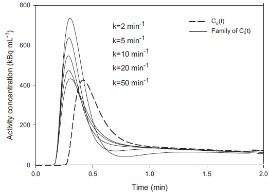
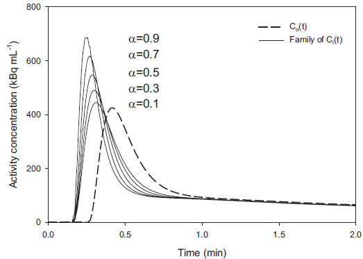
The effect of α and k on the corrected curve shape is illustrated below with two plots from [1]. The dashed line represents the dispersed, measured concentration, and the solid lines the true concentration recovered by correction.
Calibration Measurement
The parameters k and α have to be obtained from a calibration measurement with exactly the same conditions as the live experiment, i.e. with same catheter length, withdrawal speed and tracer as described in [1]. Basically, two beakers are prepared: one beaker with blood only, the other with blood and tracer (taken 1min after tracer infusion). A three-way tap is used with one catheter leading to the blood sampling system, and the other two into the beakers. Blood sampling is started with connection of the blood-only line to the detector for measuring the baseline with no radioactivity. Then the tap is switched to the catheter with blood and tracer. Correspondingly, the measured radioactivity is rising up to a constant hight. Sometime later the tap is switched back to the blood-only line, and the radioactivity is decreasing back to the baseline. Instead of the true rectangular shape of the concentration at the tap a concentration shape similar to the dispersed rectangle below [1] is measured.
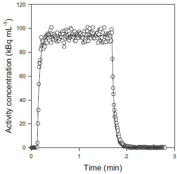
Formula can be derived [1] describing the step-up as well as the step-down edge as a function of the dispersion parameters k and α, as well as the transit time T:
Step-up:
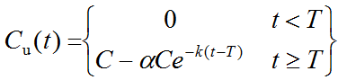
Step-down:
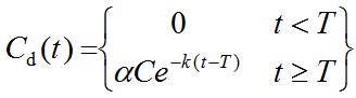
By fitting these functions to the measurement, the parameters can be determined and subsequently used in the correction of any live measurement using the same setup.
Reference
1.Munk OL, Keiding S, Bass L: A method to estimate dispersion in sampling catheters and to calculate dispersion-free blood time-activity curves. Med Phys 2008, 35(8):3471-3481. DOI