In 2010 Ito et al. introduced a new graphical method for the analysis of reversible receptor ligand binding [1]. It is applied with a plasma input curve for the calculation of the total distribution volume VT, the distribution volume of the nondisplaceable compartment VND, and therefore also allows calculation of the binding potential BPND. Furthermore, the shape of the plot gives an indication whether there the tissue includes is specific binding or not not.
Operational Model Curve
The equation of the graphical plot called is given by the equation
The following cases can be distinguished:
1.The plot is a straight line, indicating the absence of specific binding. In this case the line equation parameters have the following interpretation in terms of a 2-tissue compartment model:
a = K1 (y-intercept), b = k2 (slope), and the x-intercept equals VND.
2.The plot has a curved shape as illustrated below, indicating the presence of specific binding. In this case two regression lines are fitted to the plot: a line to the early part within a short time segment T1 to T2, and a line to the end part after an equilibration time t*. The parameters of the resulting lines can be interpreted as follows:
Early line: a1 = K1, b1 = k2, x-intercept = VND of a 2-tissue compartment model.
Late line: a2 = K1', b2 = k2', x-intercept = VT of a 1-tissue compartment model.
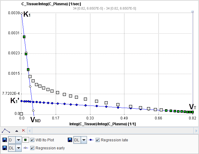
The binding potential can finally be calculated by BPND = (VT-VND)/VND
Parameter Fitting
The Ito Plot model calculates and displays the measurements transformed as described by the Ito plot formula above. It allows fitting two regression lines as follows:
1.The first regression line is fitted within the data segment specified by the times T1 and T2 (in acquisition time).
2.The second regression line is fitted to the late data segment starting at equilibration time t*.
If any of the times is changed to define a new data segment, the program finds the closest acquisition start time, fits the two regression lines, and updates the calculated parameters.
t* can be specified manually, or a value estimated using an error criterion Max Err. For instance, if Max Err. is set to 10% and the fit box of t* is checked, the model searches the earliest sample so that the deviation between the regression line and all measurements is less than 10%. Samples earlier than the t* time are disregarded for regression and thus painted in gray. Note that t* must be specified in real acquisition time, although the x-axis units are in "normalized time". The corresponding normalized time which can be looked up in the plot is shown as a non-fitable result parameter Start. In order to apply the analysis to the same data segment in all regions, please switch off the fit box of t*, propagate the model with the Copy to all Regions button, and then activate Fit all regions.
Per default, only the Ito Plot and the late regression line is shown in the curve area. However, the early regression line can also be visualized as illustrated above by enabling its box in the curve control area.
References
1.Ito H, Yokoi T, Ikoma Y, Shidahara M, Seki C, Naganawa M, Takahashi H, Takano H, Kimura Y, Ichise M et al: A new graphic plot analysis for determination of neuroreceptor binding in positron emission tomography studies. Neuroimage 2009, 49(1):578-586. DOI